Ranking Agentic Plans with a Graph World Model

The Qwen language model paper discussed how agentic environments can be simulated using world models. Agentic environments are what an LLM agent acts on: web search, terminal access, MCP servers. Simulate those and you no longer have to deploy and maintain the real infrastructure to train or test against them.

That is not what I want to talk about here. Instead of simulating the environment, think about simulating the execution itself. Can we tell whether an agent’s plan reaches the desired state, before running a single step of it?

The graph

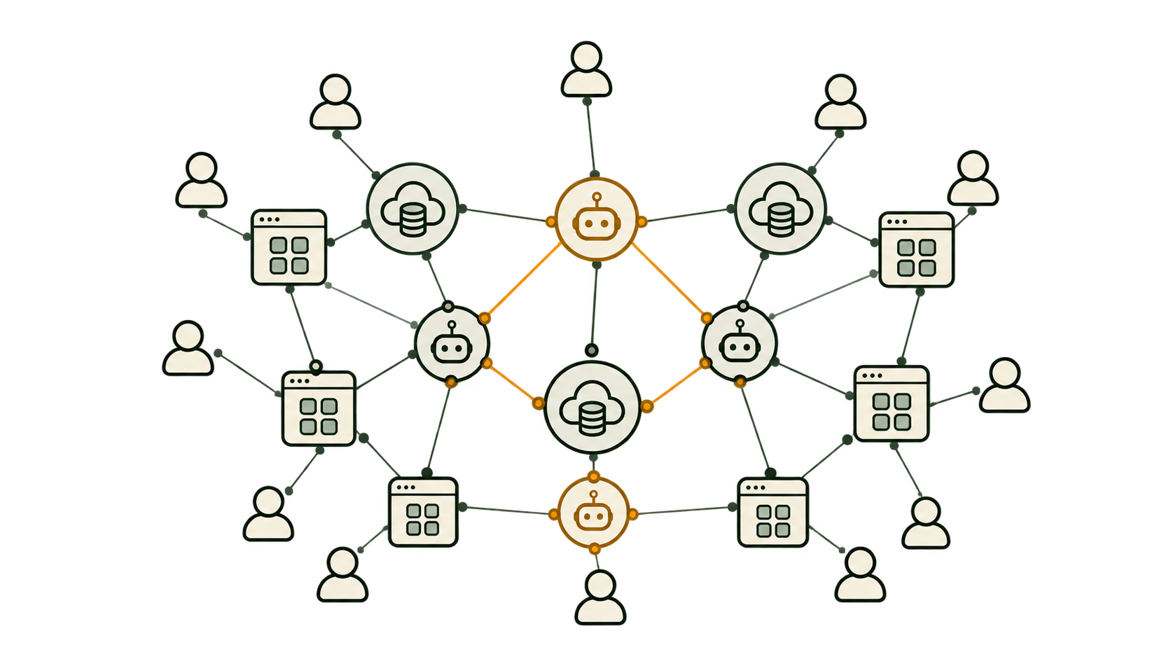
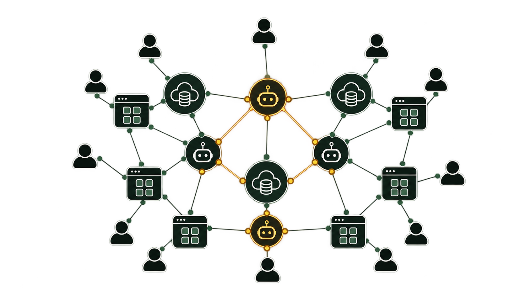
Take a coding agent. The graph at time $t$ holds:

• Nodes: a context node standing for what the agent knows right now, one node per tool it can call (read, edit, compile, test), and one node per file it is working on.
• Node features $X_t$: for a file node, does it exist, does it compile, do its tests pass, how large is it. For the context node, a latent summary of what the agent has established so far.
• Edges: which tool acts on which file, and which files depend on which.

Let’s make it simple for now assuming that the coding agent can only modify files and not create them. (I am only saying this cause I can’t explain more complicated scenarios XD.) It also makes the topology static, so this is a fixed-edge GWM: the wiring never changes across the rollout, only the numbers sitting on the nodes.

The action $a_t$ changes features of a node: which tool node fires, on which file node, with what argument. A plan is just a sequence $a_1 \dots a_T$.

Rolling the plan forward

Now feed the plan through the world model one action at a time:

$$G_0 \xrightarrow{a_1} G_1 \xrightarrow{a_2} \dots \xrightarrow{a_T} G_T$$

Two things get read off the result:

1. Does it work? A goal check on the predicted terminal graph $G_T$. For a coding agent, that means every file node compiles and every test node is green. It is binary: the plan is feasible or it isn’t.
2. What does it cost? A cost head $\hat{c}(G_t, a_t)$ emitting estimated tokens and wall time per step, summed over the rollout.

Rank the feasible plans by ascending cost. Cost only ever breaks ties between plans that actually reach the goal.

Say the planner offers two ways to do the same job:

• Plan A: write all the code at once, compile, test.
• Plan B: write a piece, compile it, test it, then integrate with what already exists and test again.

Plan A is shorter and cheaper on paper. But if the training traces say that large simultaneous edits rarely compile on the first attempt, the rollout will reflect that: $G_T$ comes back with the test node red, and Plan A is marked infeasible. Plan B costs more predicted tokens and takes more steps, but its rollout reaches a green terminal state. So Plan B wins, despite being the expensive one.

Nothing was executed to learn that. Scoring both plans cost two forward passes, not two agent runs.

Plan A — one big editPlan B — one file at a time

PrevBaselineNext

$G_0$ — before the plan

—

Baseline: everything compiles, every test is green. The task: add a --json flag to the CLI.

 

Where the training data comes from

So where does the training data come from? To train $F_\theta$ on $(G_t, a_t) \rightarrow G_{t+1}$ you need real execution traces, which is exactly the thing you were trying to avoid running.

The answer is amortization. You pay the execution cost once, up front, on a corpus of traces, and a lot of that corpus you already have, because every agent run anyone has ever logged is a sequence of tool calls and their outcomes. After that, each new plan costs a forward pass instead of a run. The cost is fixed, and the saving scales with how many plans you score against it.

ToolGrad could find an interesting use case here. Essentially, another problem is that to generate traces we need to define the tasks or prompts first, and then evaluate the traces to see whether they solved the user query optimally. But ToolGrad automates this by performing the tool operations first and then relating those tool calls back to user prompts.

The catch is that the model is only trustworthy where those traces were dense. A GWM trained on Python repositories will be confidently wrong about a Rust build. That is a real constraint on the idea.